Do Bigger Skaters Translate Better in the Playoffs?
Source:vignettes/playoff-size.Rmd
playoff-size.RmdQuestion
The playoff-size cliché is familiar: heavier teams supposedly survive the grind, win the walls, and keep scoring when space disappears. But that claim hides two different questions:
- Do bigger skaters score more in the playoffs?
- Do bigger skaters lose less scoring when regular-season hockey becomes playoff hockey?
This article uses skater_playoff_statistics(),
skater_statistics(), and players() to compare
career regular-season scoring, career playoff scoring, and the gap
between the two.
Build Player Table
We keep salary-cap-era skaters with meaningful regular-season and playoff samples. The unit is one player, not one season.
# Pull scoring and bio tables.
playoff_stats <- nhlscraper::skater_playoff_statistics()
career_stats <- nhlscraper::skater_statistics()[, c(
  'playerId',
  'rsGamesPlayed',
  'rsPoints',
  'positionCode'
)]
player_bios <- nhlscraper::players()[, c(
  'playerId',
  'playerFullName',
  'height',
  'weight'
)]

# Join player-level sources.
analysis_tbl <- merge(
  playoff_stats,
  career_stats,
  by = c('playerId', 'positionCode'),
  all.x = TRUE
)
analysis_tbl <- merge(
  analysis_tbl,
  player_bios,
  by = 'playerId',
  all.x = TRUE
)

# Keep modern skaters with stable samples.
analysis_tbl <- analysis_tbl[
  !is.na(analysis_tbl[['height']]) &
    !is.na(analysis_tbl[['weight']]) &
    analysis_tbl[['firstSeasonForGameType']] >= 20052006 &
    analysis_tbl[['gamesPlayed']] >= 20 &
    analysis_tbl[['rsGamesPlayed']] >= 200,
  ,
  drop = FALSE
]

# Fill names and compute rates.
analysis_tbl[['playerFullName']] <- ifelse(
  is.na(analysis_tbl[['playerFullName']]) |
    analysis_tbl[['playerFullName']] == '',
  paste(
    analysis_tbl[['skaterFirstName']],
    analysis_tbl[['skaterLastName']]
  ),
  analysis_tbl[['playerFullName']]
)
analysis_tbl[['regularPPG']] <-
  analysis_tbl[['rsPoints']] / analysis_tbl[['rsGamesPlayed']]
analysis_tbl[['playoffPPG']] <-
  analysis_tbl[['points']] / analysis_tbl[['gamesPlayed']]
analysis_tbl[['playoffLift']] <-
  analysis_tbl[['playoffPPG']] - analysis_tbl[['regularPPG']]
analysis_tbl[['positionBucket']] <- ifelse(
  analysis_tbl[['positionCode']] == 'D',
  'Defense',
  'Forward'
)

# Assign equal-count weight quartiles.
weight_rank <- rank(
  analysis_tbl[['weight']],
  ties.method = 'first'
) / nrow(analysis_tbl)
analysis_tbl[['weightQuartile']] <- cut(
  weight_rank,
  breaks = c(0, 0.25, 0.50, 0.75, 1),
  include.lowest = TRUE,
  labels = c('Lightest', 'Second', 'Third', 'Heaviest')
)
nrow(analysis_tbl)
#> [1] 1732
The sample has 1732 skaters. That filters out one-series mirages while still leaving enough players to compare body types.
Level Versus Translation
First, compare regular-season scoring, playoff scoring, and playoff lift by weight quartile.
# Summarize scoring by weight quartile.
quartile_summary <- aggregate(
  cbind(regularPPG, playoffPPG, playoffLift) ~ weightQuartile,
  data = analysis_tbl,
  FUN = mean
)
quartile_counts <- as.data.frame(table(analysis_tbl[['weightQuartile']]))
names(quartile_counts) <- c('weightQuartile', 'n')
quartile_summary <- merge(
  quartile_summary,
  quartile_counts,
  by = 'weightQuartile'
)
quartile_summary <- quartile_summary[
  match(levels(analysis_tbl[['weightQuartile']]), quartile_summary[['weightQuartile']]),
  c('weightQuartile', 'n', 'regularPPG', 'playoffPPG', 'playoffLift')
]
make_table(
  quartile_summary,
  caption = 'Regular-season scoring, playoff scoring, and playoff lift by weight quartile.',
  digits = 3
)| weightQuartile | n | regularPPG | playoffPPG | playoffLift | |
|---|---|---|---|---|---|
| 2 | Lightest | 433 | 0.507 | 0.458 | -0.048 |
| 3 | Second | 433 | 0.479 | 0.421 | -0.058 |
| 4 | Third | 433 | 0.436 | 0.379 | -0.057 |
| 1 | Heaviest | 433 | 0.419 | 0.378 | -0.041 |
The most important distinction is level versus translation. Lighter skaters can still post higher raw scoring rates. Bigger skaters can still translate a bit better relative to their own regular-season baseline. Those are different claims, and mixing them together is how playoff clichés become sloppy.
# Plot playoff scoring and playoff lift.
old_par <- graphics::par(no.readonly = TRUE)
graphics::par(mfrow = c(1, 2), mar = c(8, 4, 3, 1))
graphics::boxplot(
  playoffPPG ~ weightQuartile,
  data = analysis_tbl,
  col = c('#d8f3dc', '#b7e4c7', '#74c69d', '#2d6a4f'),
  border = '#1b4332',
  las = 2,
  xlab = '',
  ylab = 'Playoff Points Per Game'
)
graphics::barplot(
  quartile_summary[['playoffLift']],
  names.arg = quartile_summary[['weightQuartile']],
  col = c('#fcbf49', '#f77f00', '#d62828', '#6a4c93'),
  border = NA,
  las = 2,
  xlab = '',
  ylab = 'Playoff Lift'
)
graphics::abline(h = 0, lty = 2, col = '#495057')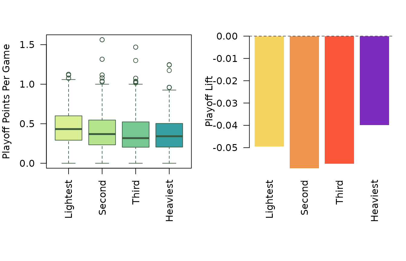
Playoff scoring level and playoff lift by weight quartile.
graphics::par(old_par)Every group loses scoring on average. The interesting question is how much.
Position Is Part of the Story
Weight and position are tangled. Defensemen are heavier, score less, and often play playoff minutes that are less offense-driven. Splitting forwards and defensemen helps keep the interpretation honest.
# Summarize rates by position and quartile.
position_summary <- aggregate(
  cbind(regularPPG, playoffPPG, playoffLift) ~ positionBucket + weightQuartile,
  data = analysis_tbl,
  FUN = mean
)
position_counts <- aggregate(
  playerId ~ positionBucket + weightQuartile,
  data = analysis_tbl,
  FUN = length
)
names(position_counts)[names(position_counts) == 'playerId'] <- 'n'
position_summary <- merge(
  position_summary,
  position_counts,
  by = c('positionBucket', 'weightQuartile')
)
make_table(
  position_summary,
  caption = 'Scoring translation by position family and weight quartile.',
  digits = 3
)| positionBucket | weightQuartile | regularPPG | playoffPPG | playoffLift | n |
|---|---|---|---|---|---|
| Defense | Heaviest | 0.307 | 0.285 | -0.022 | 197 |
| Defense | Lightest | 0.437 | 0.414 | -0.023 | 82 |
| Defense | Second | 0.384 | 0.336 | -0.048 | 142 |
| Defense | Third | 0.311 | 0.272 | -0.039 | 158 |
| Forward | Heaviest | 0.513 | 0.456 | -0.057 | 236 |
| Forward | Lightest | 0.523 | 0.468 | -0.054 | 351 |
| Forward | Second | 0.526 | 0.462 | -0.064 | 291 |
| Forward | Third | 0.507 | 0.440 | -0.067 | 275 |
The split keeps the story from becoming too neat. Size alone is not the answer. Role, position, and baseline scoring level matter.
Which Players Actually Rise?
Population averages are useful, but the player list is where the question feels like hockey.
# Show largest positive playoff lifts.
risers_tbl <- analysis_tbl[
  analysis_tbl[['gamesPlayed']] >= 40,
  c(
    'playerFullName',
    'positionBucket',
    'weight',
    'regularPPG',
    'playoffPPG',
    'playoffLift',
    'gamesPlayed'
  )
]
risers_tbl <- risers_tbl[order(-risers_tbl[['playoffLift']]), ]
risers_tbl <- utils::head(risers_tbl, 10)
make_table(
  risers_tbl,
  caption = 'Largest playoff scoring lifts among skaters with at least 40 playoff games.',
  digits = 3
)| playerFullName | positionBucket | weight | regularPPG | playoffPPG | playoffLift | gamesPlayed | |
|---|---|---|---|---|---|---|---|
| 8218 | Daniel Brière | Forward | 174 | 0.715 | 1.059 | 0.344 | 68 |
| 12706 | Evan Bouchard | Defense | 192 | 0.776 | 1.086 | 0.310 | 81 |
| 12707 | Evan Bouchard | Defense | 192 | 0.776 | 1.086 | 0.310 | 81 |
| 10827 | Jakob Silfverberg | Forward | 207 | 0.455 | 0.719 | 0.264 | 57 |
| 11958 | Sam Bennett | Forward | 193 | 0.514 | 0.766 | 0.253 | 77 |
| 11956 | Leon Draisaitl | Forward | 209 | 1.232 | 1.480 | 0.249 | 102 |
| 11957 | Leon Draisaitl | Forward | 209 | 1.232 | 1.480 | 0.249 | 102 |
| 12273 | Evan Rodrigues | Forward | 182 | 0.438 | 0.672 | 0.234 | 61 |
| 10812 | Ryan O’Reilly | Forward | 207 | 0.728 | 0.961 | 0.232 | 51 |
| 12274 | Evan Rodrigues | Forward | 182 | 0.438 | 0.667 | 0.228 | 45 |
# Show largest negative playoff lifts.
fallers_tbl <- analysis_tbl[
  analysis_tbl[['gamesPlayed']] >= 40,
  c(
    'playerFullName',
    'positionBucket',
    'weight',
    'regularPPG',
    'playoffPPG',
    'playoffLift',
    'gamesPlayed'
  )
]
fallers_tbl <- fallers_tbl[order(fallers_tbl[['playoffLift']]), ]
fallers_tbl <- utils::head(fallers_tbl, 10)
make_table(
  fallers_tbl,
  caption = 'Largest playoff scoring drops among skaters with at least 40 playoff games.',
  digits = 3
)| playerFullName | positionBucket | weight | regularPPG | playoffPPG | playoffLift | gamesPlayed | |
|---|---|---|---|---|---|---|---|
| 11439 | J.T. Miller | Forward | 211 | 0.812 | 0.400 | -0.412 | 40 |
| 8541 | Martin St. Louis | Forward | 180 | 0.911 | 0.500 | -0.411 | 44 |
| 12280 | Artemi Panarin | Forward | 176 | 1.149 | 0.761 | -0.389 | 46 |
| 11162 | Tyler Seguin | Forward | 205 | 0.813 | 0.429 | -0.384 | 42 |
| 12588 | Robert Thomas | Forward | 207 | 0.868 | 0.500 | -0.368 | 52 |
| 12589 | Robert Thomas | Forward | 207 | 0.868 | 0.500 | -0.368 | 52 |
| 12017 | Ivan Barbashev | Forward | 203 | 0.526 | 0.180 | -0.346 | 50 |
| 12748 | Noah Dobson | Defense | 200 | 0.592 | 0.250 | -0.342 | 44 |
| 10831 | John Tavares | Forward | 217 | 0.936 | 0.608 | -0.328 | 51 |
| 8675 | Brad Richards | Forward | 199 | 0.828 | 0.509 | -0.319 | 55 |
These tables are deliberately humbling. Playoff translation is not a body-type sorting machine. Some lighter players hold up beautifully. Some bigger players drop. The useful signal is a tendency, not a rule.
Model the Gap
A simple model lets us ask whether height or weight carries a standalone slope once position is included.
# Fit playoff-lift model.
lift_fit <- stats::lm(
  playoffLift ~ height + weight + I(positionCode == 'D'),
  data = analysis_tbl
)
lift_fit_tbl <- as.data.frame(summary(lift_fit)$coefficients)
lift_fit_tbl[['term']] <- rownames(lift_fit_tbl)
rownames(lift_fit_tbl) <- NULL
lift_fit_tbl[['term']] <- c(
  'Intercept',
  'Height',
  'Weight',
  'Defense indicator'
)
lift_fit_tbl <- lift_fit_tbl[, c(
  'term',
  'Estimate',
  'Std. Error',
  't value',
  'Pr(>|t|)'
)]
make_table(
  lift_fit_tbl,
  caption = 'Linear model of playoff scoring lift.',
  digits = 4
)| term | Estimate | Std. Error | t value | Pr(>|t|) |
|---|---|---|---|---|
| Intercept | 0.0088 | 0.1180 | 0.0742 | 0.9409 |
| Height | -0.0015 | 0.0020 | -0.7414 | 0.4585 |
| Weight | 0.0002 | 0.0003 | 0.7464 | 0.4555 |
| Defense indicator | 0.0274 | 0.0066 | 4.1546 | 0.0000 |
The plain-language result is that size is not magic. Once position is in the model, the direct height/weight slopes are not the headline. The playoff translation cliché is closer to a role-and-usage story than a simple bigger-is-better story.
What We Learned
Bigger skaters do not automatically become better playoff scorers. The lighter groups can still lead in raw playoff points per game. But the heaviest group can look slightly sturdier relative to its own regular-season scoring baseline.
That split answer is the point. nhlscraper makes it easy
to combine career stats and player bios, but the interpretation still
has to respect the shape of the data. A good mini research question is
not always one where the cliché is true or false. Sometimes the best
answer is: true in one sense, false in another.